FAST-LIO with loop closing on IGNIS-8

What this post covers#

If you have been following the IGNIS-8 project, you know the vehicle has no steering wheel and no GPS for the kind of centimetre-level pose a battery reconnaissance robot needs indoors. The answer is the same one modern quadruped and warehouse robots use: fuse a fast IMU with a 3D LiDAR into an odometry estimate that tracks position, attitude and velocity in three dimensions. This post walks through that system end to end:

• The error-state Kalman filter (ESKF) — how a 250 Hz IMU propagates a 15-dimensional state and how the point cloud corrects it.
• The local voxel map and plane fit — how scan points become measurement constraints, and the gates that keep the update safe in an open, structure-poor hall.
• Loop closing — keyframes, geometric detection, point-to-plane confirmation, pose-graph optimisation, and the map rebuild that follows.
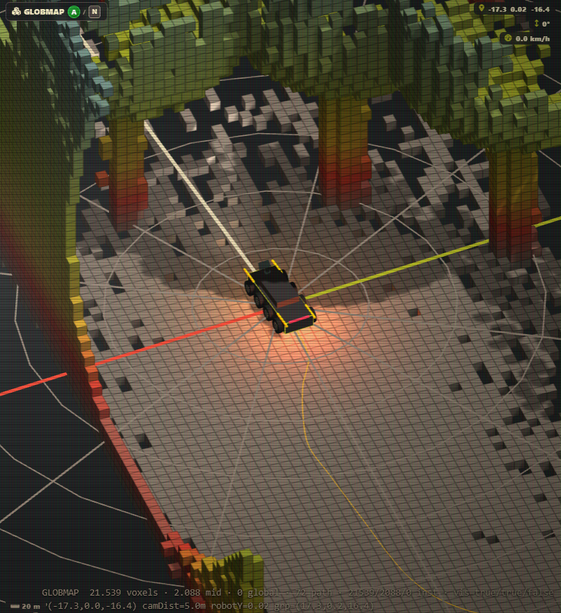
• The three-level 3D voxel map the operator sees in the GLOBMAP view, and how a loop rebuilds it without drift.
• Software diagrams for the whole pipeline.

The tone is the same as the other IGNIS-8 posts: concrete, code-level, and honest about what is still simulation-only.

A quick look at the hardware#

The L1 PM is a solid-state LiDAR with an upward-pointing hemispherical scan. On IGNIS-8 it is mounted at the front of the chassis, tilted 45° forward, so that upward hemisphere dips below the horizon ahead and covers the near field in front of the vehicle. It also contains an IMU. Two numbers matter:

• The IMU reports raw gyroscope and accelerometer samples at 250 Hz.
• The point cloud arrives as a full scan at 20 Hz — roughly 12 ms between scans.

The mismatch between 250 Hz and 20 Hz is exactly why a filter is needed: between two scans the IMU must carry the pose. The LIO consumes every IMU sample directly (never polling, never dropping), integrates it into the filter, and lets the next scan correct whatever the integration drifted.

The sensor's points are reported in its own tilted frame. Before anything touches the LIO, the driver's normalizeMount rotates each point by the 45° mount pitch back into the vehicle frame (+X right, +Y up, −Z forward). The LIO therefore integrates vehicle-frame points directly — the same frame the simulation produces, so the whole pipeline is exercised identically in the simulator and on hardware.

flowchart TD
    subgraph SENSOR["Sensor"]
        IMU[IMU 250 Hz<br/>raw gyro + accel]
        L1[L1 PM LiDAR<br/>upward hemisphere, 45° forward tilt]
    end

    subgraph DRIVER["LiDAR driver (single producer goroutine)"]
        DEC[decode + normalizeMount<br/>own-structure + range filter]
        TAPS[scan tap + IMU tap]
    end

    subgraph LIO["pkg/lio — ESKF core"]
        PRED[Predict<br/>IMU propagates state + 15×15 cov]
        UPD[UpdateScan<br/>point-to-plane residuals<br/>against local voxel map]
        LOOP[Loop closing<br/>keyframes, scan-match,<br/>pose-graph optimisation]
    end

    subgraph MAP["globalMapTask — 3-level voxel map"]
        LVL[local 0.125 m · mid 0.25 m · coarse 0.5 m<br/>sliding cylindrical windows, upsampling]
        WS[stream /ws/lio_map<br/>visible slice only]
        REBUILD[ReplaceWorld after a loop]
    end

    HMI[HMI GLOBMAP<br/>3D voxels + pose]

    IMU --> DEC
    L1 --> DEC
    DEC --> TAPS
    TAPS --> PRED
    TAPS --> UPD
    PRED --> UPD
    UPD --> LOOP
    LOOP -->|CorrectedWorld| REBUILD
    TAPS --> LVL
    LVL --> WS
    REBUILD --> WS
    WS --> HMI
    LIO -->|6DOF pose + velocity| HMI

The pipeline at a glance#

The diagram above shows the whole perception stack. Reading left to right:

1. The LiDAR driver decodes the raw sensor stream, normalises the mount tilt, filters own-structure and range, and hands the accepted points to two consumers via taps.
2. The LIO task (lio_task.go) feeds every IMU sample and every scan into pkg/lio. The LIO's ESKF predicts with the IMU and corrects with the scan against a local map. It publishes the 6-DOF pose and velocity.
3. The global map task (globalMapTask) builds the environment model from the LIO pose and the scan tap: a three-level voxel map that the HMI shows as 3D voxels.
4. When loop closing accepts a revisit, the LIO publishes the corrected keyframe world (CorrectedWorld) and the global map rebuilds both levels (ReplaceWorld), so the operator sees a drift-free environment.

Two details matter for concurrency. The LIO is not safe for concurrent use, and the two taps run in the driver's single producer goroutine — the supervisor in simulation, the read loop on hardware — so the core is race-free by construction. The published pose is guarded by its own mutex for the WebSocket and other consumers.

The error-state Kalman filter#

An error-state Kalman filter splits the state into a nominal part that the IMU propagates and an error part that the measurements correct. The idea is older than FAST-LIO, but FAST-LIO popularised it for LiDAR-inertial fusion because it keeps the correction linear and small even though the attitude lives on a manifold.

The 15-dimensional error state#

The filter tracks a nominal state and a 15-dimensional error vector:

Block	Error	Meaning
0–2	δθ	attitude error (rotation vector)
3–5	δp	position error
6–8	δv	velocity error
9–11	δb_g	gyroscope bias error
12–14	δb_a	accelerometer bias error

The nominal state itself carries the attitude quaternion Q, position P, velocity V, and the two IMU biases. The world frame points +Y up, so gravity acts along −Y.

Predict — the IMU drives the nominal state#

Each raw IMU sample (gyro ω, accel a) advances the nominal state:

Q ← Q ⊗ Δq( (ω − b_g) · dt )
a_world = R(Q) · (a − b_a) − g
P ← P + V·dt + ½·a_world·dt²
V ← V + a_world·dt

The covariance predict is the linearised propagation P ← F·P·Fᵀ + Q, where F is built from the discrete error dynamics — the skew of the gyro, the rotation of the accelerometer skew, and the bias-error couplings. The process noise Q is a diagonal simplification driven by the IMU noise densities and the bias random walks.

Match — the scan becomes point-to-plane constraints#

A scan arrives at 20 Hz. First the points are range-filtered (0.2–15 m). Then, at the predicted pose, each point is transformed into the world frame and matched against the local map: the map points within 0.5 m are gathered and a plane is fitted to them. The signed distance of the query point from that plane is the measurement residual. The plane fit is cached per point so the iterated update runs it once, not once per iteration.

Update — the residuals correct the state#

The ESKF update is applied per point as a scalar Kalman gain — avoiding the m×m matrix inversion of a batch update. Each point contributes a measurement Jacobian H (1×15) that maps the residual onto the error state, and the state plus covariance are updated with the standard Kalman equations. The update is iterated a couple of times so the linearisation catches up with the correction.

The update is gated, and that is what makes it safe#

The interesting engineering is not the math but the gates around it. An LIO in an open hall with only a floor, a ceiling and a ramp has very little planar structure, and a naive update can walk the pose off even at the exact pose. The LIO defends against that at four levels:

1. Per-point Mahalanobis gate — a point whose innovation lies more than MaxInnovationSigma (4σ) standard deviations from zero is an outlier (a wrong plane, a moving object, a spurious hit) and is skipped.
2. Scan-level gate — if fewer than MinPlanePoints points matched, or the mean absolute innovation exceeds MaxMeanInnovation (0.05 m), the whole scan is rejected. It does not correct the state, but it is still inserted into the map so the map grows into unexplored geometry.
3. Observability weighting — each point's measurement noise is inflated when its plane normal points along a direction the scan only weakly observes. In an open hall the floor and ceiling observe the vertical strongly, but the horizontal directions carry little planar structure; an unweighted update would let the biased plane fits walk the pose sideways. The weighting confines the correction to the well-observed directions and lets the IMU own the rest.
4. Trust region — a scan that would move the pose more than MaxScanCorrectionM (0.05 m) or change the velocity more than 0.05 m/s is rejected as a whole and the state rolls back to the prediction. Such a large correction cannot come from a consistent map.

The same gates protect the loop closing, which is why loop closing can be left enabled even in the degenerate simulation.

flowchart TD
    A["1 · Predict (IMU, 250 Hz)<br/>nominal state Q, P, V, biases<br/>15x15 covariance P = F P F^T + Q<br/>(gravity -Y)"] --> B["Scan in (20 Hz)<br/>range filter 0.2-15 m,<br/>vehicle-frame points"]

    B --> C["2 · Assessment pass<br/>plane-fit each point vs map<br/>gather neighbours, fit plane (gates)<br/>observability matrix A = sum(n n^T)<br/>planes cached"]

    C --> G["Quality gate<br/>matched >= MinPlanePoints<br/>mean innovation <= MaxMeanInnovation<br/>observability diagonal > 0"]

    G -->|"reject"| A
    G -->|"pass"| D["3 · Iterated update<br/>per point: Mahalanobis gate,<br/>observability-weighted noise,<br/>bounded by trust region"]

    D --> E["4 · Insert scan<br/>register at corrected pose<br/>(rejected scans still insert)"]

    C -. "match / fit" .-> M["Local voxel map<br/>0.2 m voxels, one point per voxel<br/>match radius 0.5 m<br/>sliding window +/-20 m / +/-8 m<br/>prune gated on motion"]

    E -. "corrected pose" .-> M
    M --> C

The local voxel map#

The local map is a downsampled cloud of world-frame points: one representative per 0.2 m voxel, keeping the point nearest the voxel centre so the map stays sharp. For a query point, the map gathers the points in the neighbouring voxel layers that fall within the 0.5 m match radius and fits a plane to them.

The plane fit is a PCA on the cluster: centroid, covariance, eigenvalues. The normal is the eigenvector of the smallest eigenvalue; the centre is the cluster centroid; the residual is the signed distance of the query point from that plane. Three gates decide whether the cluster is a usable plane:

• Curvature — the ratio of the smallest to the largest eigenvalue must be below MaxCurvature (0.1). A blob has no thin direction and yields no constraint.
• Spread — the ratio of the middle to the largest eigenvalue must be above MinSpread (0.1). A cluster that is thin in two directions is a line, not a plane.
• One-sidedness — the centroid must not lie too far from the query point (MaxCentroidOffset, 0.2 × match radius). A cluster whose centroid is far away comes from an occlusion boundary, a curved object or the leading edge of the map, and its plane is biased.
• Surface roughness — the RMS deviation of the gathered points from the fitted plane must stay below MaxSurfaceRoughness (0.02 m). A curved surface makes the fitted plane systematically tilt, biasing every residual on it.

The map is a sliding window around the current pose — ±20 m horizontal, ±8 m vertical — so it stays bounded on a long drive. Pruning is an O(n) scan over the voxels, so it only runs once the vehicle has moved at least a quarter of the window since the last pass.

flowchart TD
    A["Gather neighbours<br/>query point to world frame<br/>collect map points within<br/>MatchRadiusM = 0.5 m<br/>(voxel layers covering the radius)"] --> B["Fit plane (PCA)<br/>centroid, covariance, eigenvalues<br/>normal = smallest eigenvector<br/>centre = cluster centroid<br/>residual z = n·(p - c)"]

    B --> G["Valid plane?"]
    G -->|"reject"| R["Rejection gates<br/>fewer than MinPlanePoints (5)<br/>curvature too high (blob, min/max eigenvalue)<br/>spread too low (line)<br/>centroid too far from query<br/>surface roughness too high<br/>(curved surface gives biased plane)"]
    G -->|"accept"| C["Plane constraint (n, c) to ESKF update<br/>per-point Mahalanobis gate,<br/>observability weight"]
    C --> W["Observability weighting<br/>noise proportional to dominant info / per-axis info"]

    A -. "gather" .-> M["Local voxel map<br/>0.2 m cells, one point per voxel"]

Loop closing: fixing the drift#

Even a well-gated LIO drifts. The IMU biases and the scan-to-map residuals accumulate a pose error that grows with the driven distance — centimetres per hundred metres, depending on the environment. For a vehicle that drives a loop through a battery hall, that drift is the difference between coming back to a spot that looks right and coming back to one that is visibly off.

Loop closing attacks the problem directly: when the vehicle revisits an area it has seen before, the system corrects the accumulated drift against the earlier geometry. The implementation is a keyframe-based pose graph with a geometric candidate test and a scan-match confirmation.

Keyframes: the odometry chain#

A keyframe is the pose plus a voxel-downsampled body-frame scan, recorded whenever the vehicle has travelled KeyframeDistM (4 m) or turned by KeyframeYawRad (0.6 rad ≈ 34°) since the last one. The first scan is always a keyframe. The chain of keyframes 0…n is the odometry graph — each consecutive pair is a constraint that ties the poses together, trusting the relative motion recorded at scan time.

Downsampling the scan per keyframe keeps the memory bounded: the body-frame points are voxel-quantised at the LIO's voxel size (0.2 m), keeping one representative per voxel nearest the voxel centre. The keyframe also stores the scan in the world frame at the recorded pose, which is what later rebuilds the corrected global map.

Detection: which earlier keyframe is a candidate?#

When a new keyframe is added, the closer scans the earlier keyframes for geometric candidates. An earlier keyframe is a candidate if:

• its horizontal position lies within LoopRadiusM (8 m) of the current keyframe, and
• its heading differs by no more than LoopYawRad (±90°), and
• it is at least LoopMinIndexGap (10) keyframes back.

The index gap matters: consecutive keyframes share most of their geometry by construction, so a loop must be a revisit separated by a real path, not the vehicle still standing at the same spot. The oldest qualifying candidate wins.

Confirmation: a scan match that cannot lie#

A geometric candidate alone proves nothing — the vehicle could be near its old track without actually seeing the same walls. So the candidate is confirmed by a point-to-plane scan match:

1. A tiny local voxel map is built from the candidate keyframe's world points.
2. The current body-frame scan is transformed by the predicted relative pose (from the odometry chain) into the candidate's world frame.
3. Each scan point is matched to a plane in that tiny map; the point-to-plane residuals are evaluated.

The match is accepted only when at least 30 % of the scan points find a plane and the mean residual stays below 0.04 m. Both thresholds are conservative: a loop is a global statement, so it must be very consistent. Additionally, the correction a loop would apply is bounded by LoopMaxCorrectionM (2 m) — a match that would yank the vehicle by more than that is a false positive and is skipped.

Pose-graph optimisation#

Once a loop is accepted, a loopConstraint links the revisited keyframe a to the current one b with the measured relative pose. The pose graph is then optimised:

• The odometry constraints between consecutive keyframes keep the chain rigid — the relative motion recorded at scan time is trusted.
• The loop constraint says the measured relative pose (from the scan match) must hold.
• The difference between the chained and the measured relative pose is the accumulated drift. Distributing it over the keyframes between a and b — weighted towards the newest keyframe — spreads the correction across the path instead of yanking only the current pose.

The rotation error is applied as a small rotation-vector correction per keyframe, scaled by the same distribution weight. The graph is small (tens of keyframes) and the drift it corrects is small (centimetres to a few decimeters), so this distributed correction is a robust approximation of the full least-squares solution.

After the optimisation the current pose follows the corrected newest keyframe, so the odometry continues from the loop-closed pose. ConsumeLoop resets the result so the caller that acts on it — the map rebuild — runs exactly once per accepted loop, not once per scan.

flowchart TD
    KF["New keyframe?<br/>accumulate dist + yaw<br/>dist at least 4 m OR |yaw| at least 0.6 rad"]
    KF -->|"no"| WAIT["wait for next scan"]
    KF -->|"yes"| DET["Loop detection<br/>for each earlier keyframe, at least 10 back:<br/>horizontal dist at most 8 m<br/>heading diff at most 90 deg<br/>candidate (oldest wins)"]

    DET --> MATCH["Confirm by scan match<br/>tiny voxel map from candidate<br/>current scan at predicted relative pose<br/>point-to-plane match<br/>accept if frac at least 30 % and<br/>mean residual at most 0.04 m"]

    MATCH -->|"no"| NOLOOP["no loop"]
    MATCH -->|"yes"| CON["Add loop constraint<br/>bounded: correction at most 2 m"]

    CON --> OPT["Pose-graph optimisation<br/>odometry chain rigid; loop pulls<br/>the revisit back; weight towards newest<br/>translation at most 2 m, small rotation"]

    OPT --> CORR["Correct current pose<br/>odometry continues from loop pose"]
    CORR --> REBUILD["Map rebuild<br/>CorrectedWorld to ReplaceWorld<br/>HMI shows drift-free voxels"]

    REBUILD -->|"next scan"| KF

The map rebuild#

The point of loop closing is not the pose graph alone — it is that the map the operator sees no longer carries the drift. After an accepted loop, CorrectedWorld() returns the world points of all keyframe scans at their corrected poses, and the caller feeds that into globalMapTask.ReplaceWorld, which clears both map levels and rebuilds them from the corrected cloud. The GLOBMAP view therefore snaps to the drift-free environment after a revisit — the walls the operator saw when the vehicle first passed now line up with the walls seen on the second pass.

The three-level voxel map#

The operator never sees the raw point cloud in the GLOBMAP view — they see a voxel map. The globalMapTask builds it from the LIO pose and the scan tap. It has three levels so a large area stays available without the memory or the stream exploding:

Level	Cell	Window	Role
LOCAL (fine)	0.125 m	±10 m (20×20×10 m)	every scan lands here; detail up close
MID (medium)	0.25 m	±30 m	local voxels upsample here (~7–15 m)
GLOBAL (coarse)	0.5 m	±100 m (200×200×10 m)	mid voxels upsample here (>15 m)

When a local voxel leaves the local window it is not dropped — it is upsampled into the mid level (addCoarseLocked, keeping the point nearest the coarse voxel centre) and survives at reduced resolution. Mid voxels that leave the mid window are upsampled into the coarse level. Voxels that leave the coarse window are pruned: the far side loses data as the vehicle moves.

The windows are cylindrical around the pose: a voxel leaves a level once its horizontal (XZ) distance from the pose exceeds the window half-extent. This matches the radial resolution bands the HMI draws, so the detail coarsens on a circle around the robot rather than on a square — corner voxels no longer linger in a fine level they are not displayed in.

flowchart TD
    LOCAL["LOCAL (fine)<br/>0.125 m cells<br/>±10 m window (20×20×10 m)<br/>every scan lands here<br/>detail up close"]
    MID["MID (medium)<br/>0.25 m cells<br/>±30 m window<br/>local voxels upsample here<br/>7-15 m"]
    GLOBAL["GLOBAL (coarse)<br/>0.5 m cells<br/>±100 m window (200×200 m)<br/>mid voxels upsample here<br/>over 15 m"]

    LOCAL -->|"leave window"| MID
    MID -->|"leave window"| GLOBAL

    PRUNE["Pruning — cylindrical windows<br/>a voxel leaves a level once its horizontal<br/>(XZ) distance from the pose exceeds the<br/>window half-extent — matches the HMI's<br/>radial resolution bands"]
    STREAM["Stream to the HMI (/ws/lio_map)<br/>local in full; mid/global only the slice<br/>within the client's view radius<br/>after a loop: ReplaceWorld rebuilds<br/>all levels from corrected keyframes"]

    GLOBAL --> PRUNE
    PRUNE --> STREAM

Streaming and the view radius#

The stream (/ws/lio_map) carries the local level in full and the mid/global levels only the slice within the view radius the client reports — JSON text messages like {"view": 25.0}. The HMI computes its visible extent from the orbit camera and re-sends it when the operator zooms. A 200×200 m map never ships as a ~38 MB frame; the server sends only what the operator can actually see. After a loop, ReplaceWorld rebuilds all three levels from the corrected keyframes, so the drift-free environment is what streams next.

The 45° mount and the coordinate frames#

The L1 PM's upward hemisphere becomes useful for a ground robot only because of the 45° forward mount. normalizeMount rotates the raw sensor-frame points back into the vehicle frame before they reach the LIO, so the LIO integrates vehicle-frame points directly. The simulation produces vehicle-frame points already (the mount pitch there only shapes the ray directions; the trace hits are back-rotated by toSensor), so the hardware path and the simulation path agree on the frame — which is what lets the whole LIO and loop-closing stack run identically in the simulator and on the real sensor.

Two coordinate facts keep the pipeline honest:

• The vehicle frame is +X right, +Y up, −Z forward, origin at the sensor head.
• The world frame of the LIO points +Y up; a body point p is placed in the world by R(Q)·p + P.

The attitude published to the HMI is decomposed from the world-from-body quaternion into yaw (positive = left), pitch (positive = nose up) and roll.

Why the demo disables scan matching#

There is one deliberate exception worth explaining. newLioTask sets UseScanMatching = false for the simulation. The reason is that the simulated hall is a degenerate case: with only the floor, the ceiling and the ramp as planar structure, the horizontal directions are almost unobservable, and the few biased plane fits hold the position at the ramp entrance against the IMU. There the pure IMU integration is the accurate source.

On hardware, where the IMU drifts and the environment has real structure, scan matching stays available and safe through the defaults — the gates, the observability weighting and the trust region keep it from walking off. Loop closing, in contrast, is enabled everywhere: its own scan-match gates and the bounded correction keep it safe even in the degenerate simulation, and on hardware it corrects the drift when the vehicle revisits an area. The keyframes in the simulation produce few or no loops because the deterministic path rarely returns, but the machinery is exercised end to end.

How the pieces fit together (one scan cycle)#

Putting it all together, one 20 Hz scan does the following:

1. The driver decodes the scan, normalises the mount, filters, and hands the accepted points to the LIO tap.
2. The LIO predicts with every IMU sample that arrived since the last scan (250 Hz worth of propagation).
3. UpdateScan assesses the scan against the local map at the predicted pose: plane fits, observability matrix, quality gates.
4. If the scan passes, the iterated update corrects state and covariance, bounded by the trust region.
5. The scan is inserted into the local map at the corrected pose.
6. If loop closing is enabled, the corrected pose and scan go to the loop closer: a keyframe decision, candidate search, scan-match confirmation, and — on an accepted loop — pose-graph optimisation plus the map rebuild.
7. The published pose feeds the HMI telemetry and the global map task.

The whole cycle runs in a single goroutine, so there is no locking inside the LIO core itself — only the published pose and the global map snapshot carry their own mutexes for the WebSocket consumers.

Tests#

pkg/lio is covered by unit tests that pin down the behaviour this post describes:

• Config validation — every parameter is range-checked so a bad config fails loudly at construction.
• The ESKF update — the state and covariance respond correctly to a point-to-plane residual.
• The plane-fit gates — curvature, spread, one-sidedness and surface roughness reject the wrong clusters.
• The keyframe trigger — distance and yaw thresholds fire new keyframes.
• The loop candidate test — the geometric tests (radius, yaw, index gap) accept the right candidates and reject the wrong ones.
• The point-to-plane loop match — including an offset candidate pose, proving the match confirms a real revisit.
• The pose-graph correction — the drift distributes across the chain and the correction stays bounded.

The VCU task tests drive the simulated vehicle and verify the LIO pose follows the motion, including the ramp pitch in the odometry and the attitude. All tests are green.

Status and next steps#

Everything in this post is software that runs today in the simulation. The LIO fuses the simulated IMU and scans, loop closing exercises its keyframe and match machinery, and the three-level voxel map renders in the GLOBMAP view with the radial resolution bands and the loop rebuild path.

The remaining work is hardware:

• Real LiDAR bring-up — connect the L1 PM, verify the decode and the mount normalisation against real point clouds, and tune the IMU noise and bias-walk parameters from real data.
• Loop-closing tuning — confirm the keyframe density and match thresholds on a real hall, where the geometry is richer than the simulation.
• Field verification — drive a real loop and check that the pose comes back and the map rebuilds without drift.

The short version: a FAST-LIO-style ESKF fuses the IMU and the LiDAR into a 6-DOF pose, gates and observability weighting keep it honest in structure-poor rooms, and a keyframe-based loop closer detects revisits, confirms them by scan match, optimises the pose graph and rebuilds the three-level voxel map without drift.

Function-by-function tour of pkg/lio#

The package is deliberately small and readable. Beyond the orchestrator LIO, the ESKF math, the local map and the loop closer each live in their own file. This section walks every exported function and what it does, in the order the data flows.

The orchestrator — lio.go#

New(cfg) validates the configuration and constructs the LIO with an identity state, an identity 15×15 covariance, a fresh local map and a fresh loop closer. Reset() discards state, covariance, map and keyframes — used when the vehicle is repositioned or a new mission starts. It is the same as constructing a new LIO, which keeps the reset path trivial to reason about.

State() and Pose() are the read accessors: the full 15-dimensional state (attitude quaternion, position, velocity, both biases) and the position + attitude pair. MapSize() returns the number of points in the local map, which stays bounded thanks to the sliding window. LastScan() and LastLoop() return the diagnostics of the most recent scan update and loop pass. ConsumeLoop() returns the loop result and clears it, so a caller that rebuilds the map runs exactly once per accepted loop rather than once per scan — the loop result would otherwise be re-read at every 20 Hz scan.

Predict(gyro, accel, dt) is the IMU entry point: it advances the nominal state and the covariance. UpdateScan(points) is the scan entry point: range filter, assessment, gated iterated update, map insertion, and the loop-closing pass. Both are called from lio_task.go; because the driver's taps run in a single goroutine, they never overlap.

SetCorrectedPose(p, q) applies a loop-closed pose: after the pose graph is optimised, the newest keyframe's pose moved, and the live state follows it so the next scans and IMU samples integrate from the corrected pose.

The filter — eskf.go#

predictNominal(s, gyro, accel, dt, cfg) is the discrete integration shown above: the quaternion is pre-multiplied by the rotation of the gyro reading (minus bias) over dt, the accelerometer reading (minus bias) is rotated into the world frame and gravity is subtracted, and position and velocity are integrated.

predictCovariance(P, s, gyro, accel, dt, cfg) builds the Jacobian F from the continuous error dynamics and returns F·P·Fᵀ + Q. The interesting blocks are the attitude-error couplings: −[ω]×dt between the attitude error and itself, −dt into the gyro-bias error, +dt from velocity error into position error, −R[a]×dt from attitude error into velocity error, and −R·dt from accel-bias error into velocity error. The process noise Q is a diagonal simplification with the IMU noise densities and the bias random walks as the standard deviations per square root of time.

updatePoint(s, P, pBody, n, c, r, sigma) is the heart of the correction. It computes the world-frame position of the body point, the signed residual to the plane, the 1×15 measurement Jacobian H (the attitude block is −nᵀ·R·[pBody]×, the position block is nᵀ), the innovation covariance S = H·P·Hᵀ + r, applies the Mahalanobis gate, computes the Kalman gain, and updates all seven error-state blocks via the shared scalar innovation −z. Finally P ← (I − K·H)·P.

The local map — map.go#

addPoint(p) inserts a world point into its voxel, keeping the point nearest the voxel centre so the map stays sharp. addScan(points, s) transforms a body-frame scan into the world frame and inserts it. match(pBody, s) is the plane fit: it gathers the map points within MatchRadiusM, applies the gates, fits the plane by eigen-decomposition and returns normal + centre. prune(pose) drops points outside the sliding window, gated on the motion since the last pass.

The loop closer — loop.go#

newLoopCloser(cfg) starts an empty closer. add(s, scan, cfg) is the per-scan entry point: it accumulates the distance and yaw since the last keyframe, decides whether a new keyframe is due, stores it (both body-frame and world-frame downsampled), runs detect(), and optimises when a loop was accepted. detect() scans the earlier keyframes for candidates, confirms them by matchScan, and adds the best accepted constraint. candidate(cur, can) applies the geometric tests (radius, heading, index gap). matchScan(scan, can, rel) builds the tiny map and evaluates the point-to-plane match. optimize(res) distributes the drift over the chain. CorrectedWorld() returns the loop-closed world points for the map rebuild. Count() and Reset() are diagnostics and lifecycle.

The full configuration table#

Every parameter of the LIO is configurable and validated at construction. The table lists the factory defaults and what each one does:

Parameter	Default	Purpose
GravityM	9.81	local gravity, world frame +Y up
ImuNoiseGyro	0.003	gyro noise density (rad/s per √Hz)
ImuNoiseAccel	0.06	accel noise density (m/s² per √Hz)
GyroBiasWalk	0.0001	gyro bias random walk (per √s)
AccelBiasWalk	0.001	accel bias random walk (per √s)
MeasurementNoise	0.01	per-point plane-residual variance
MinRangeM / MaxRangeM	0.2 / 15.0	accepted scan range
VoxelSizeM	0.2	local map voxel edge
MatchRadiusM	0.5	neighbour radius for plane fit
MapWindowM	20.0	horizontal map window half-extent
MapWindowY	8.0	vertical map window half-extent
MinPlanePoints	5	minimum neighbours for a plane
MaxCurvature	0.1	blob/plane separation
MinSpread	0.1	line/plane separation
MaxCentroidOffset	0.2	one-sided cluster gate (× radius)
MaxSurfaceRoughness	0.02	plane flatness gate (m)
MinObservability	0.02	per-axis info floor
MaxScanCorrectionM	0.05	trust-region position bound
MaxScanVelocityCorr	0.05	trust-region velocity bound
Iterations	2	iterated update passes
MaxInnovationSigma	4.0	per-point Mahalanobis gate (σ)
MaxMeanInnovation	0.05	scan-level gate (m)
KeyframeDistM	4.0	keyframe distance trigger
KeyframeYawRad	0.6	keyframe yaw trigger
LoopRadiusM	8.0	loop candidate radius
LoopMinIndexGap	10	min keyframe separation
LoopYawRad	π/2	max heading difference
LoopMaxCorrectionM	2.0	loop correction bound
LoopMatchMinFrac	0.3	min matched fraction for a loop
LoopMaxMeanInnovation	0.04	loop match residual bound

Validate() range-checks all of them and returns ErrInvalidConfig (wrapped) so a bundled errors.Is check catches a bad configuration at startup — a common source of subtle failures in real-world deployments.

Why an ESKF and not something simpler#

The question naturally arises: why not a plain pose integration, or a particle filter, or a full factor graph? The answer is a combination of accuracy, robustness and cost:

• A pure IMU integration drifts. Without an absolute reference, the double-integrated accelerometer wanders quadratically. The ESKF keeps the bias errors as state and lets the LiDAR observations correct them.
• A full factor graph is heavy. Optimising every scan against every landmark is expensive and unnecessary at 20 Hz. The ESKF keeps a compact Gaussian belief and only the loop layer builds a graph, and only over keyframes (a few dozen).
• The error-state form is well conditioned. Because the correction is always small, the linearisation stays valid and the attitude update avoids the singularities of Euler-angle parametrisations.

This is the same reasoning that made FAST-LIO popular: the filter does the cheap, continuous work at IMU rate, the scan does the sparse, corrective work at LiDAR rate, and everything is bounded so the system is safe in environments it has not been tuned for.

The observability weighting, explained with a picture#

The observability weighting is subtle enough to deserve its own explanation. The normal information matrix A = Σ n·nᵀ over all matched points captures how much directional information a scan carries. Its diagonal is the information along each world axis.

Consider an open hall. The floor and ceiling provide plenty of horizontal planes, whose normals point mostly up — so the vertical axis has huge information. The ramp and the distant walls provide a little horizontal information, but far less. Without weighting, a single biased plane fit on a curved object could dominate the horizontal correction and walk the pose sideways. The LIO therefore computes, for each point, the least-observed axis the point's normal touches, and inflates the measurement noise by the ratio of the dominant to that axis's information. A point whose plane normal points purely along a weakly observed direction is downweighted almost to zero; the IMU integration owns that direction instead.

The floor MinObservability (0.02) stops the weight from vanishing entirely on a badly structured scan, and the trust region (MaxScanCorrectionM) is the final backstop. The net effect: the filter trusts the scan exactly where the scan is informative, and leans on the IMU exactly where it is not. That is the property that makes the update safe to leave enabled in the general case.

flowchart TD
    SCAN["Scan arrives (20 Hz)<br/>each point has a fitted plane normal n"]
    SCAN --> A["Build the observability matrix<br/>A = sum over all points of n * n^T<br/>(3x3, accumulates per scan)"]
    A --> DIAG["Read the diagonal of A<br/>= how much info the scan carries<br/>per world axis"]
    DIAG -->|"Y: floor + ceiling<br/>huge info"| TRUST["Trust the scan fully:<br/>weight w close to 1<br/>noise stays r = r"]
    DIAG -->|"X, Z: ramp + walls<br/>little info"| DOWN["Downweight the scan:<br/>w = diag[weak] / diag[strong]<br/>noise r = r / w becomes large"]
    TRUST --> OUT["Result: the filter follows<br/>the scan where it is informative"]
    DOWN --> OUT
    OUT --> SAFE["and leans on the IMU where it is not<br/>MinObservability 0.02 keeps w above zero,<br/>trust region (MaxScanCorrectionM) as backstop"]

The sliding window, the pruning, and why the map stays bounded#

A map that grows forever is a leak. Every new scan adds points; without a bound, a long mission accumulates unbounded memory and the plane-fit neighbourhood scans grow quadratically. The local map's sliding window solves it: points farther than MapWindowM (20 m) in X or Z, or MapWindowY (8 m) vertically, are pruned.

Pruning is O(n) over the voxels, so it is gated on motion: it only runs once the vehicle has moved at least a quarter of the window since the last pass. The scan range (15 m) bounds how far the sensor can add points, so a 20 m window keeps every point the matching can use while bounding the memory on a long drive. The same idea scales to the global map, where the three levels and their cylindrical windows keep a 200×200 m map available without a 38 MB stream.

flowchart TD
    SCAN["Every scan inserts points<br/>into the local map"]
    SCAN --> GROW["Without a bound the map<br/>would grow forever"]
    GROW -->|"moved less than 1/4 window<br/>since the last pass"| WAIT["Skip the prune pass<br/>(it is O(n) over the voxels)"]
    GROW -->|"moved at least 1/4 window<br/>since the last pass"| PRUNE["Prune pass over the voxels<br/>drop every point outside the window"]
    PRUNE --> HOR["horizontal: X or Z beyond<br/>MapWindowM (20 m) -> pruned"]
    PRUNE --> VER["vertical: Y beyond<br/>MapWindowY (8 m) -> pruned"]
    HOR --> KEEP["scan range 15 m < window 20 m:<br/>every point the matching can<br/>still use is kept"]
    VER --> KEEP
    KEEP --> BOUND["the map memory stays bounded<br/>on a long drive"]

Telemetry the operator can actually read#

The LIO publishes more than a pose. ScanStats (from LastScan()) reports how many points the scan contained after the range filter, how many found a plane, the mean absolute innovation at the predicted state, whether the update was applied, and the net position correction. LoopResult (from LastLoop() / ConsumeLoop()) reports the number of keyframes, how many candidates were evaluated, how many passed the scan match, whether a loop was accepted, the net correction, and the mean residual of the accepted match.

For an operator at the HMI this turns a black box into a diagnosable system: a scan that is never applied (Applied = false) signals a structure-poor or inconsistent environment; a loop result with a growing Candidates count but no Accepted tells you the thresholds are too strict or the geometry is ambiguous; a Correction near the LoopMaxCorrectionM bound warns that the loop is barely within tolerance. The telemetry is also what makes the tuning loop on real hardware tractable — you can see exactly why a loop was or was not accepted before changing a threshold.

Loop closing: the worst case, the false positive#

A loop that is accepted but wrong is worse than no loop at all: it would yank the map sideways and corrupt the environment model. The design defends against this in depth:

• The geometric candidate test already rejects most false positives — an area that is far away or viewed from the wrong direction is never even matched.
• The point-to-plane confirmation requires 30 % of the scan to agree with the candidate's map at a mean residual below 0.04 m. A genuine revisit sees the same walls from the same heading, so the residuals are tiny; a coincidental proximity does not produce that.
• The correction bound (LoopMaxCorrectionM, 2 m) is the final gate. A drift error worth correcting is centimetres to a few decimeters; a match that would move the pose by 2 m is, by definition, not a drift error. It is skipped, and the odometry keeps its prediction.
• The trust region of the scan update applies even inside the loop match: a loop match that would move the current pose beyond the bound is rejected.

The net result is a loop closer that is conservative by construction. In the simulation, the deterministic path produces few or no loops — which is exactly what the design intends: loop closing is there to catch real revisits on hardware, not to fire on coincidental proximity.

How the whole stack is tested#

The tests fall into three groups. Unit tests in pkg/lio pin down the filter: lio_test.go covers config validation, the ESKF update, the plane-fit gates, and the keyframe trigger; loop_test.go covers the loop candidate test, the point-to-plane loop match (including an offset candidate pose), and the pose-graph correction. The VCU task tests drive the simulated vehicle and verify the LIO pose follows the motion, including the ramp pitch in the odometry and the attitude decomposition. All of it runs on every build and stays green.

The simulation is not a toy: it produces vehicle-frame scans from the same ray-casting the hardware driver produces, so the LIO and loop-closing code paths run identically on simulated and real data. The one deliberate difference — scan matching off in the simulation, on by default for hardware — is documented in the code and explained above.

What the operator sees#

On the HMI, the LIO shows up in two ways. The GLOBMAP view renders the three-level voxel map, with the radial resolution bands (fine within ~7 m, mid to ~15 m, coarse beyond) reflecting the three levels. The attitude and velocity readouts in the HUD come from the published pose: yaw, pitch, roll, and the three velocity components. On a real battery hall, the operator watches the GLOBMAP fill in as the vehicle drives, sees the walls snap together after a loop, and reads the pose directly from the attitude values — no odometry wheel to be fooled by.

The map itself is streamed over /ws/lio_map with the 76-byte wire header carrying the pose and the per-level cell sizes, counts and height bounds, followed by the voxel payloads and the driven path. The client reports its view radius as text messages, and the server sends only the slice that fits — the same streaming discipline that keeps the 200×200 m map usable on a live connection.

A walk through one concrete scenario#

Imagine the vehicle starts at the entrance of a battery hall, drives down the left aisle, around a rack island, and comes back up the right aisle past the entrance.

1. At boot the LIO is at the identity state. The first scan is range-filtered, matched against an empty map (no planes yet, no correction), and inserted — the map now contains the entrance.
2. As the vehicle drives down the left aisle, keyframes accrue every 4 m or 34° of yaw. The local map fills with the rack faces, the floor and the ceiling. The ESKF corrects the pose against these planes at 20 Hz; the observability weighting keeps the horizontal corrections honest.
3. Around the rack island the vehicle turns, the pose tracks the pitch and roll of the floor, and new keyframes are recorded on the turn.
4. Coming up the right aisle, the vehicle approaches the entrance area again. A new keyframe lands within 8 m of the first keyframes, with a matching heading and an index gap well above 10. The candidate test fires.
5. The current scan is matched against the candidate's tiny map at the predicted relative pose. The walls of the entrance agree; 30 % of the points find planes at a mean residual below 0.04 m. The loop is accepted.
6. The pose graph distributes the drift (say 15 cm accumulated around the loop) over the keyframes between the two ends, weighted towards the newest. The current pose follows the corrected newest keyframe.
7. The caller consumes the loop result and calls ReplaceWorld. The global map is rebuilt from the corrected keyframe scans; the GLOBMAP view snaps the entrance back into alignment. From the operator's chair, the map that had quietly drifted a few centimetres now lines up again — and the HUD pose reflects the correction immediately.

The whole sequence is automatic. The operator does nothing but drive; the LIO and loop closer do the bookkeeping.

Known limits and honest caveats#

No system is free. The loop closer as written is a two-keyframe loop constraint with a distributed correction — it is not a full multi-loop optimiser like a pose-graph SLAM with bundle adjustment. For a battery hall that is the right trade-off: the correction it applies is bounded, cheap and good enough to remove the visible drift. If IGNIS-8 ever needs global consistency across many revisits over a long mission, the keyframe structure is already there; extending optimize to a least-squares solver over all constraints would be the natural next step.

The scan matching is deliberately disabled in the simulation because the hall is too degenerate for it to help. On hardware it comes back on, and the tuning of the noise and bias-walk parameters against real data is still on the list. The loop thresholds (30 % matched fraction, 0.04 m residual) are conservative by design; the real hall will tell us whether they are conservative enough or too conservative.

Finally, the whole LIO runs in a single goroutine by design. It is not thread-safe, and the driver's single-producer design is what makes that safe. Any future consumer that wants to call Predict or UpdateScan from another goroutine would have to serialise access — the published pose and the map snapshot already carry their own locks.

A short FAQ#

Q: Why 250 Hz IMU and 20 Hz LiDAR? 
A: The L1 PM reports the IMU at 250 Hz and a full scan at 20 Hz. The filter needs the fast IMU to carry the pose between scans; the slow scan corrects the drift. Both are inherent to the sensor, and the LIO is designed around exactly that mismatch.

Q: What does the 45° mount change? 
A: Without it, the upward hemisphere would see only the ceiling and the sky. Tilted 45° forward, it covers the near field in front of the vehicle — the walls, the floor ahead, the racks. normalizeMount rotates the points back into the vehicle frame so the LIO sees a normal ground-robot point cloud.

Q: Can the LIO work without loop closing? 
A: Yes. It is a separate layer (UseLoopClosing, off by default in the config factory). The core ESKF odometry runs without it; loop closing only adds the keyframe bookkeeping and the correction pass. The VCU task enables it because the gates make it safe everywhere.

Q: What happens when the scan is rejected? 
A: The state keeps the prediction, the scan is still inserted into the map (so the map grows into new areas), and the telemetry reports Applied = false. The next scan tries again from the corrected-by-IMU state.

Q: How is this different from the old 2.5D SLAM? 
A: The 2.5D SLAM projected the world onto a flat grid and tracked only position and heading. The LIO tracks the full 6-DOF pose — position, attitude, velocity — so ramps and inclines are solved in three dimensions instead of being flattened. The 2.5D SLAM has since been removed from the codebase; the LIO plus the three-level voxel map is the sole perception source.

Status and next steps (recap)#

Everything in this post is software that runs today in the simulation: the ESKF odometry, the gated scan update, the loop closer with its keyframe and match machinery, and the three-level voxel map with the radial bands and the loop rebuild path. The remaining work is hardware bring-up and tuning, as described earlier.

If you want the short version of this whole post: a FAST-LIO-style error-state Kalman filter fuses the IMU and the LiDAR into a 6-DOF pose; gates and observability weighting keep it honest in structure-poor rooms; and a keyframe-based loop closer detects revisits, confirms them by scan match, optimises the pose graph and rebuilds the three-level voxel map without drift. That is the perception core IGNIS-8 will drive on.